Dipoles

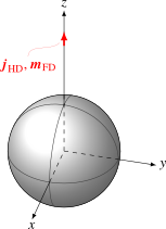
Setup for the excitation with a Hertzian or a Fitzgerald dipole.

Definition

The dipoles are defined as infinitesimal time harmonic current elements. Note that the definitions differ from the ones employed in [Jac99, pp. 411ff] basically by a factor of $k$. Hence, they lead to different static fields, i.e., for $k\rightarrow 0$.

Hertzian Dipole

The Hertzian dipole with dipole length $l$, electric current $I$, and orientation $\hat{\bm p}$ at position $\bm r_0$ is assumed to have the current density

\[\bm{j}_\mathrm{HD} = Il \hat{\bm p} \delta (\bm r - \bm r_0) \,,\]

where $\delta$ denotes the Dirac delta distribution.

Fitzgeral Dipole

The Fitzgerald (magnetic) dipole with dipole length $l$, magnetic current $M$, and orientation $\hat{\bm p}$ at position $\bm r_0$ is assumed to have the current density

\[\bm{m}_\mathrm{FD} = Ml \hat{\bm p} \delta (\bm r - \bm r_0) \,.\]

API

The API provides the following constructors with default values:

SphericalScattering.HertzianDipole — Type

ex = HertzianDipole(
        embedding   = Medium(ε0, μ0),
        frequency   = error("missing argument `frequency`"),
        amplitude   = 1.0,
        position    = error("missing argument `position`"),
        orientation = SVector{3,typeof(frequency)}(0.0, 0.0, 1.0),
)

source

SphericalScattering.FitzgeraldDipole — Type

ex = FitzgeraldDipole(;
        embedding   = Medium(ε0, μ0),
        frequency   = error("missing argument `frequency`"),
        amplitude   = 1.0,
        position    = error("missing argument `position`"),
        orientation = SVector{3,typeof(frequency)}(0.0, 0.0, 1.0),
)

source

Tip

The orientation vector is automatically normalized to a unit vector during the initialization.

Radiated Field

The electric field of the Hertzian dipole itself (without scatterer) is [Jac99, pp. 411ff]

\[\bm e(\bm r) = Z_\mathrm{F} \cfrac{Il}{4 \pi} \mathrm{e}^{-\mathrm{j} k r} \left( \cfrac{k}{r} ((\hat{\bm n} \times \hat{\bm p}) \times \hat{\bm n}) + \left(\cfrac{1}{k r^3} + \cfrac{\mathrm{j}}{r^2} \right) (3 \hat{\bm n} (\hat{\bm n} \cdot \hat{\bm p}) - \hat{\bm p}) \right)\]

with $Z_\mathrm{F} = \sqrt{\mu / \varepsilon}$ and the magnetic field

\[\bm h(\bm r) = \cfrac{Il}{4 \pi} \cfrac{\mathrm{e}^{-\mathrm{j} k r} }{r} \left(k + \cfrac{1}{\mathrm{j} r} \right) (\hat{\bm n} \times \hat{\bm p})\]

where

\[\hat{\bm n} = \cfrac{\bm r - \bm r_0}{|\bm r - \bm r_0|}\,.\]

Note

The fields of the Fitzgerald dipole follow from the duality relations.

API

The general API is employed:

E  = field(ex, ElectricField(point_cart))

H  = field(ex, MagneticField(point_cart))

FF = field(ex, FarField(point_cart))

Scattered Field

The scattered field computation is a generalization of the analysis in [Jin15, pp. 374ff]. For the magnetic dipole duality relations are employed. The series and their evaluation are described under Electromagnetic Spheres.

Tip

For the scattered field computation the orientation of the dipole is restricted: the dipole has to be perpendicular to the surface of the sphere.

This can be achieved, e.g., by defining the orientation first

orientation = normalize(SVector(0.0,1.0,1.0))

and then setting the position as a multiple of the orientaion:

position = 2.0 * orientation

API

The general API is employed:

E  = scatteredfield(sp, ex, ElectricField(point_cart))

H  = scatteredfield(sp, ex, MagneticField(point_cart))

FF = scatteredfield(sp, ex, FarField(point_cart))

Total Field

API

The general API is employed:

E  = field(sp, ex, ElectricField(point_cart))

H  = field(sp, ex, MagneticField(point_cart))

FF = field(sp, ex, FarField(point_cart))