Coordinate System

Spherical Coordinates

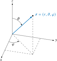
The employed coordinate system uses the following convention for the spherical coordinates everywhere in the code with $\vartheta \in [0, \pi]$ and $\varphi \in [-\pi, \pi]$.

Oblate Spheroidal Coordinates

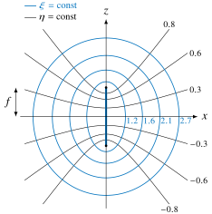
The oblate spheroidal coordinates $(\xi, \eta, \varphi)$ with $\xi \ge 0$, $\eta \in [-1, 1]$ and $\varphi \in [-\pi, \pi]$ are defined by

\[x = f \sqrt{(1 + \xi^2)(1 - \eta^2)} \cos \varphi \,, \qquad y = f \sqrt{(1 + \xi^2)(1 - \eta^2)} \sin \varphi \,, \qquad z = f \xi \eta\]

where $f$ denotes the semifocal distance, so that the distance from the origin is $r = f \sqrt{\xi^2 + 1 - \eta^2}$.

The surface $\xi = \xi_0$ is an oblate spheroid with equatorial radius $f \sqrt{1 + \xi_0^2}$ and polar radius $f \xi_0$; the surfaces $\eta = \mathrm{const}$ are the confocal one-sheeted hyperboloids. The coordinate $\eta$ thus plays the role of $\cos \vartheta$ and reduces to it in the limit of large $\xi$, whereas $\varphi$ is the azimuth of the spherical coordinates.

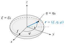
The figure shows the spheroid $\xi = \xi_0$ together with the focal ring of radius $f$ in the plane $z = 0$ (dotted). In the meridian plane of a point, the coordinate line $\eta = \eta_0$ is a branch of the confocal hyperbola, which starts on the focal disc and crosses the spheroid at a right angle.

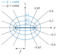
In the $xz$-plane, the coordinate lines are confocal ellipses ($\xi = \mathrm{const}$) and hyperbolas ($\eta = \mathrm{const}$), shown above for $f = 1$. The ellipse $\xi = 0$ degenerates into the focal disc $|x| \le f$ (thick line), the hyperbolas $\eta = \pm 1$ into the $z$-axis, and $\eta = 0$ into the plane $z = 0$ outside the disc.

Two degenerate cases are of interest. For $\xi_0 \rightarrow \infty$ the spheroid approaches a sphere, with $f \rightarrow 0$ such that $f \xi_0$ stays finite, and the coordinates degenerate. For $\xi_0 = 0$ the surface collapses onto the disc of radius $f$ in the plane $z = 0$, its two faces being distinguished by the sign of $\eta$: inside the disc, the sign of $\eta$ cannot be recovered from the Cartesian coordinates of a point.

The metric coefficients read

\[h_\xi = f \sqrt{\cfrac{\xi^2 + \eta^2}{1 + \xi^2}} \,, \qquad h_\eta = f \sqrt{\cfrac{\xi^2 + \eta^2}{1 - \eta^2}} \,, \qquad h_\varphi = f \sqrt{(1 + \xi^2)(1 - \eta^2)} \,.\]

Since $\hat{\bm e}_\xi = h_\xi^{-1} \partial \bm r / \partial \xi$ is the outward normal of the surface $\xi = \mathrm{const}$, the normal derivative is $\partial / \partial n = h_\xi^{-1} \partial / \partial \xi$.

These coordinates are employed for the oblate acoustic spheroid and the disc. The conversions are available as SphericalScattering.obl2cart, SphericalScattering.cart2obl, SphericalScattering.oblateMetric and SphericalScattering.oblateBasis.

Prolate Spheroidal Coordinates

The prolate spheroidal coordinates $(\xi, \eta, \varphi)$ with $\xi \ge 1$, $\eta \in [-1, 1]$ and $\varphi \in [-\pi, \pi]$ are defined by

\[x = f \sqrt{(\xi^2 - 1)(1 - \eta^2)} \cos \varphi \,, \qquad y = f \sqrt{(\xi^2 - 1)(1 - \eta^2)} \sin \varphi \,, \qquad z = f \xi \eta\]

where $f$ denotes the semifocal distance, so that the distance from the origin is $r = f \sqrt{\xi^2 - 1 + \eta^2}$.

The surface $\xi = \xi_0$ is a prolate spheroid with equatorial radius $f \sqrt{\xi_0^2 - 1}$ and polar radius $f \xi_0$, the latter being the larger one; the surfaces $\eta = \mathrm{const}$ are the confocal two-sheeted hyperboloids. As for the oblate coordinates, $\eta$ reduces to $\cos \vartheta$ in the limit of large $\xi$.

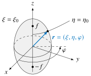
The figure shows the spheroid $\xi = \xi_0$ together with its foci $z = \pm f$ on the axis. In the meridian plane of a point, the coordinate line $\eta = \eta_0$ is a branch of the confocal hyperbola, which starts on the axis between the foci and crosses the spheroid at a right angle.

In the $xz$-plane, the coordinate lines are confocal ellipses ($\xi = \mathrm{const}$) and hyperbolas ($\eta = \mathrm{const}$), shown above for $f = 1$. The ellipse $\xi = 1$ degenerates into the segment $|z| \le f$ between the foci (thick line), the hyperbolas $\eta = \pm 1$ into the parts $|z| \ge f$ of the $z$-axis, and $\eta = 0$ into the plane $z = 0$.

The two degenerate cases mirror those of the oblate coordinates. For $\xi_0 \rightarrow \infty$ the spheroid approaches a sphere, with $f \rightarrow 0$ such that $f \xi_0$ stays finite. For $\xi_0 = 1$ the surface collapses onto the segment of the axis between the foci, $|z| \le f$, which is not supported as a scatterer.

The metric coefficients read

\[h_\xi = f \sqrt{\cfrac{\xi^2 - \eta^2}{\xi^2 - 1}} \,, \qquad h_\eta = f \sqrt{\cfrac{\xi^2 - \eta^2}{1 - \eta^2}} \,, \qquad h_\varphi = f \sqrt{(\xi^2 - 1)(1 - \eta^2)} \,,\]

the outward normal of the surface $\xi = \mathrm{const}$ again being $\hat{\bm e}_\xi = h_\xi^{-1} \partial \bm r / \partial \xi$.

These coordinates are employed for the prolate acoustic spheroid. The conversions are available as SphericalScattering.prol2cart, SphericalScattering.cart2prol, SphericalScattering.prolateMetric and SphericalScattering.prolateBasis.